| Atomic Bomb Survivors [II] Chromosome aberration analysis 1983-1985 (METEX Collaboration Study) |
This study was performed by a collaborative study funded by MEXT Scientific Research Grant (#58380019 for 1983-1985) on “Dose assessment of A-bomb radiation by chromosome aberrations”.
![]()
| Members of collaborative study Awa, A. (Rad Effects Res Foundation) Abe, S. (Hokkaido University) Ejima, Y. (Kyoto University) Furuyama, J. (Hyogo Medical College) Hayata, I. (National Inst Radiol Sci) |
Hirai, M. (University of Tokyo) Honada, T. (Rad Effects Res Foundation) Ichimaru, M. (Nagasaki University) Ikushima, T. (Kyoto University) Ishii, Y. (Osaka University) Ishihara, T. (National Inst of Radiol Sci) |
Kamada, N. (Hiroshima University) Kishi, K. (Kyorin University) Kodama, S. (Kyoto University) Matsubara, S. (Tokyo Med Dent Univ) Sadamori, N. (Nagasaki University) Sasaki, M. S. (Kyoto University) (*Charman) |
Sofuni,
T. (National Inst. Of Health Sci) Sonta, S. (Aichi Birth Defects Res Inst) Takatsuji, T. (Nagasaki University) Tatsumi, J. (Nagasaki University) Tezuka, H. (National Inst Genetics) Tsuji, H. (National Inst Radiol Sci) |
Categories
in the table:
Subject ID: Hiroshima (H), Nagasaki (N); Sex: Male (M), Female (F), ATB: Age (yrs) at the time of bombing, Shielding: No shielding (0), Japanese wooden house (2), Concrete building (3), Shaded
by concrete building (4)
Acute symptoms: Burn (B), Diarrhea (D), Fever (F), Epilation (E)
| . | |||||||||||||||||||||||||||||
| No | Subject | Date of | Sex | Age | Distance | Shielding | Symptoms | No. of | Aberrations | Cells | Distribution of cells with Dic+Ring | ||||||||||||||||||
| ID | sampling | (ATB) | (km) | cells | Tri | Dic | Rc | Ra | aM | F | del | S | del | X1Cu | X2Cu | Cs | 0 | 1 | 2 | 3 | 4 | 5 | 6 | ||||||
| 1 | ABH03001 | 1983.09.09 | M | 26.4 | 0.57 | 1 | F | 1,508 | 0 | 16 | 3 | 2 | 39 | 17 | 4 | 4 | 3 | 17 | 5 | 35 | 1,491 | 16 | 2 | 1 | |||||
| 2 | ABH03002 | 1983.09.09 | M | 20.0 | 0.95 | 1 | EDBF | 1,664 | 0 | 8 | 1 | 1 | 63 | 14 | 4 | 2 | 2 | 16 | 1 | 57 | 1,654 | 10 | |||||||
| 3 | ABH03003 | 1983.09.12 | M | 19.6 | 0.95 | 0 | EDBF | 1,531 | 0 | 13 | 1 | 3 | 228 | 14 | 4 | 1 | 1 | 15 | 5 | 194 | 1,517 | 12 | 1 | 1 | |||||
| 4 | ABH03004 | 1983.09.12 | F | 16.5 | 0.80 | 3 | - | 1,730 | 0 | 12 | 3 | 0 | 21 | 17 | 4 | 3 | 3 | 17 | 2 | 16 | 1,716 | 1 | |||||||
| 5 | ABH03005 | 1983.09.12 | F | 25.0 | 1.24 | 3 | - | 1,741 | 0 | 8 | 4 | 3 | 17 | 16 | 5 | 2 | 2 | 19 | 3 | 14 | 1,725 | 15 | 1 | ||||||
| 6 | ABN04004 | 1983.09.22 | F | 17.0 | 0.70 | 4 | EDF | 1,800 | 0 | 11 | 2 | 2 | 20 | 17 | 8 | 5 | 3 | 20 | 5 | 16 | 1,786 | 14 | |||||||
| 7 | ABN04009 | 1983.09.29 | M | 18.8 | 1.50 | 0 | BF | 1,700 | 0 | 1 | 0 | 0 | 6 | 5 | 3 | 0 | 0 | 5 | 0 | 5 | 1,699 | 1 | |||||||
| 8 | ABN04012 | 1983.10.06 | M | 5.9 | 1.40 | 1 | - | 1,700 | 0 | 7 | 0 | 1 | 11 | 5 | 2 | 0 | 0 | 6 | 4 | 11 | 1,692 | 8 | |||||||
| 9 | ABN04013 | 1983.10.06 | F | 18.9 | 1.50 | 1 | ED | 1,800 | 0 | 5 | 3 | 0 | 11 | 8 | 3 | 2 | 2 | 10 | 2 | 9 | 1,792 | 8 | |||||||
| 10 | ABN04014 | 1983.10.06 | M | 19.4 | 1.20 | 0 | EDF | 1,800 | 0 | 4 | 1 | 0 | 43 | 6 | 3 | 4 | 3 | 10 | 1 | 38 | 1,795 | 5 | |||||||
| 11 | ABH05013 | 1983.10.21 | M | 14.5 | 0.85 | 0 | EDBF | 1,975 | 1 | 3 | 1 | 3 | 215 | 11 | 8 | 9 | 8 | 18 | 1 | 187 | 1,967 | 7 | 1 | ||||||
| 12 | ABH05016 | 1983.11.16 | F | 25.5 | 0.80 | 1 | EDBF | 1,941 | 0 | 16 | 2 | 5 | 65 | 31 | 15 | 4 | 4 | 28 | 2 | 60 | 1,922 | 16 | 2 | 1 | |||||
| 13 | ABN06019 | 1983.10.13 | F | 0.9 | 0.90 | 0 | ED | 1,900 | 1 | 5 | 0 | 1 | 64 | 6 | 2 | 0 | 0 | 3 | 3 | 61 | 1,987 | 2 | 1 | ||||||
| 14 | ABN06045 | 1983.12.08 | M | 36.1 | 1.50 | 0 | - | 2,000 | 0 | 12 | 3 | 2 | 36 | 21 | 8 | 7 | 6 | 21 | 1 | 33 | 1,984 | 15 | 1 | ||||||
| 15 | ABN06049 | 1983.12.15 | M | 16.2 | 1.40 | 0 | EBF | 1,916 | 0 | 9 | 0 | 0 | 38 | 12 | 7 | 1 | 1 | 12 | 4 | 36 | 1,909 | 6 | 1 | ||||||
| 16 | ABN06032 | 1983.11.17 | F | 11.9 | 1.00 | 1 | D | 1,200 | 0 | 4 | 3 | 0 | 9 | 8 | 2 | 1 | 1 | 10 | 0 | 9 | 1,193 | 7 | |||||||
| 17 | ABH06029 | 1984.04.18 | F | 25.9 | 1.60 | 1 | - | 1,525 | 0 | 0 | 1 | 0 | 11 | 2 | 1 | 2 | 2 | 4 | 0 | 11 | 1,522 | 1 | |||||||
| 18 | ABH07001 | 19.85.03.02 | M | 26.4 | 0.93 | 1 | EDF | 1,250 | 0 | 4 | 0 | 0 | 65 | 9 | 6 | 4 | 4 | 12 | 1 | 61 | 1,246 | 4 | |||||||
| 19 | ABH07002 | 1985.03.02 | F | 23.1 | 0.93 | 1 | EDF | 1,000 | 0 | 0 | 1 | 0 | 41 | 3 | 3 | 1 | 1 | 4 | 1 | 40 | 999 | 1 | |||||||
| 20 | ABN08001 | 1985.04.10 | M | 15.8 | 1.80 | 1 | EDB | 1,600 | 0 | 5 | 0 | 1 | 9 | 8 | 4 | 2 | 2 | 11 | 1 | 9 | 1,594 | 6 | |||||||
| 21 | ABN08002 | 1985.04.10 | M | 20.9 | 1.20 | 1 | E | 1,500 | 0 | 0 | 0 | 1 | 8 | 2 | 2 | 0 | 0 | 3 | 0 | 7 | 1,499 | 1 | |||||||
| 22 | ABN08003 | 1985.04.10 | M | 29.6 | 1.40 | 3 | D | 1,500 | 0 | 0 | 0 | 1 | 7 | 0 | 0 | 0 | 0 | 1 | 0 | 6 | 1,499 | 1 | |||||||
| 23 | ABN08004 | 1985.04.10 | M | 25.2 | 0.69 | 3 | - | 1,500 | 1 | 1 | 1 | 0 | 21 | 2 | 1 | 1 | 1 | 3 | 1 | 18 | 1,498 | 2 | |||||||
| . | |||||||||||||||||||||||||||||
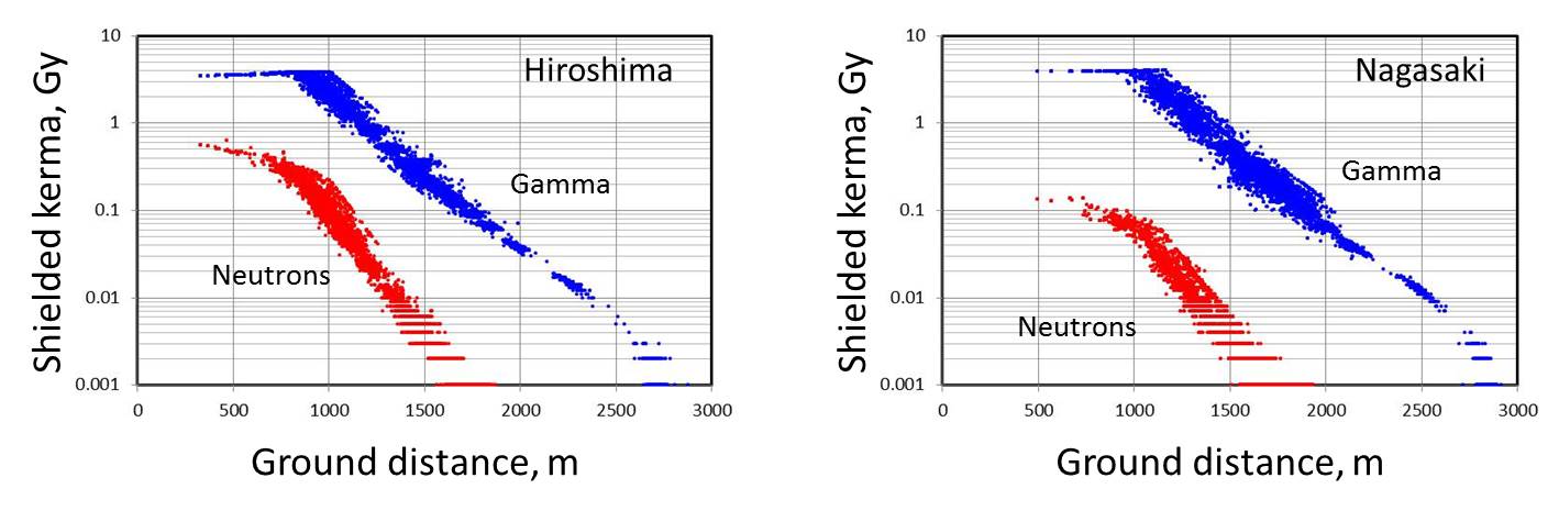
| Parameters of Bombing | DS02 free-in-air shielded kerma (Gy) for RERF survivor cohorts, modified from “lss13mort” data of RERF (http://rerf.org.jp) |
| Hiroshima Bomb type: Little boy (Uranium type) Bombing: August 6, 1945; 8:15 a.m. Burst height: 600±20 m Energy yield: 16±2 kt Nagasaki Bomb type: Fat man (Plutonium type) Bombing: August 9, 1945; 11:02 a.m. Burst height: 503±10 m Energy yield: 21±2 kt |
 |
| Testing for the uniformity of chromosome scoring among scorers |
|
Currently, the inter-laboratory collaborative
studies are often organized for chromosome aberration analysis of the radiation
exposed persons, especially for those supposed to be exposed to low-level
radiation where large scale data analysis is needed for the dose evaluation,
or those involved in radiation accident where there is an immediate need
for the biological dose assessment. In such collaborative study, the variability
or uniformity of the results obtained by individual scorer is always a
matter of important concern. We developed the statistical method for the
assessment of variability of the participants
of the collaborative analysis. p1=p2 The number of aberrations, a, in the number of cells scored, n, follow a binomial distribution, B(a2:n2,p2) for K B(a1:n1,p1) for N-1. The statistical test for p of the two binomial distributions may be possible by assuming that, under the null hypothesis, a2 follows the hypergeometric distribution. That is, with a=a1+a2 and n=n1+n2, the probability density follows the hypergeometric function p(a2)=p(a2:n2,a,n)=[comb(a; a2)comb(n-a;n2-a2)]/comb(n;n2)
Then, the lower tail probability of a2 is LP=sum[i-0 to a2] p(i) And the upper tail probability of a2 is LP=sum[i=a2 to n2] p(i) 2) Uniformity test for the scoring efficiency
in multiple samples Similarly, PSU(x) is obtained for the sum of UP being below probability density of x. If the PSL or PSU are below significance level (i.g., 0.005), the scoring of the scorer K is significantly different from that of averaged efficiency of the rest of scorers. If the PSL is blow significance level, the scorer K shows significantly underscore. If the PSU is blow the significance level, the scorer K shows significantly overscore as compared to the average of the rest of scorers. 3) Results and implication for the issue of
overdispersion |
| . | ||||||||||||||||||||||||||||
| Scorer | Probability | X1Cu-cells | Cs-cells | Scorer | Probability | X1Cu-cells | Cs-cells | Scorer | Probability | X1Cu-cells | Cs-cells | Scorer | Probability | X1Cu-cells | Cs-cells | |||||||||||||
| A | upper | 54.0 | - | 6.1 | - | E | upper | 81.6 | - | 100 | ↓ | I | upper | 98.9 | ↓ | 98.7 | ↓ | M | upper | 17.4 | - | 95.4 | ↓ | |||||
| lower | 47.0 | 85.6 | lower | 27.1 | 0 | lower | 0.9 | 0.3 | lower | 84.4 | 1.7 | |||||||||||||||||
| B | upper | 14.1 | - | 0 | ↑ | F | upper | 1.4 | ↑ | 3.4 | ↑ | J | upper | 42.4 | - | 99.3 | ↓ | N | upper | 88.9 | ↓ | 99.5 | ↓ | |||||
| lower | 89.7 | 100 | lower | 98.5 | 99.3 | lower | 58.7 | 2.4 | lower | 3.0 | 0.8 | |||||||||||||||||
| C | upper | 30.1 | - | 0 | ↑ | G | upper | 54.3 | - | 0 | ↑ | K | upper | 94.3 | - | 99.9 | ↑ | O | upper | 84.9 | - | 2.6 | ↑ | |||||
| lower | 71.0 | 100 | lower | 50.5 | 100 | lower | 11.9 | 0 | lower | 31.1 | 97.5 | |||||||||||||||||
| D | upper | 8.9 | - | 96.0 | ↓ | H | upper | 85.5 | - | 99.0 | ↓ | L | upper | 25.4 | - | 0.2 | ↑ | P | upper | 83.5 | - | 90.3 | ↓ | |||||
| lower | 88.9 | 1.7 | lower | 30.3 | 0 | lower | 67.4 | 100 | lower | 8.5 | 3.6 | |||||||||||||||||
| [↑]: Sum of upper tail probability is significantly small (over-score) | ||||||||||||||||||||||||||||
| [↓]: Sum of lower probability is significantly small (under-score) | ||||||||||||||||||||||||||||
| [ - ]: No significant at 5% level. | ||||||||||||||||||||||||||||
| . | ||||||||||||||||||||||||||||